Machine Learning – Supervised – Linear Regression

Introduction

Machine Learning is broadly classified into two types :

•  Supervised Learning
• Unsupervised Learning

Supervised Learning

In supervised learning, we will have our input and output variables defined and we ask the machine to learn from the existing data and use that learning on unseen/future data for prediction.

For example, let’s consider we have data for a diabetes problem in which we have two input variables height and weight and the output variable is whether the patient is diabetic or not. Now we will train our algorithm on the input variables (x) and output variable (y). And when a new patient gives her/his weight and height the algorithm will be able to predict whether that patient is diabetic or not.

This is a classic and basic example of a supervised classification algorithm.

Supervised Learning is in turn classified into :

1. Regression
2. Classification

In this article/blog we will discuss Linear Regression – The Theory in detail.

Linear Regression

Before getting into the topic we will see what is regression?

When the output variable is numeric/continuous then it’s a Regression problem whereas when the output variable is categorical then it’s Classification.

Linear regression is one of the simplest, oldest, and important algorithms. This is the first algorithm that every data scientist/analyst and ML engineer will learn. It’s famous and significant because of the interpretability which the model offers.

Linear regression is classified into :

• Simple Linear Regression : When there is one input variable and one output variable then we call it simple linear regression
• Multiple Linear Regression : When there is more than one input variable and one output variable then we call it multiple linear regression

Working of Linear Regression

Let’s learn about simple linear regression (SLR) and multiple linear regression (MLR). MLR is just an extension of SLR.

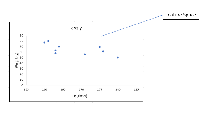
In SLR, the algorithm will first do a scatter plot between one input variable and one output variable. Then it will fit a line that minimizes the distance between each of the points in the feature space and the line.

For example, let’s say we take data where we have to predict the weight for the given height of the person.

Process of Identifying the best fit line

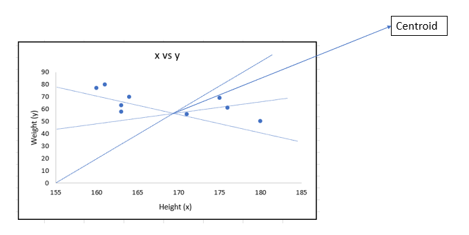
1. Find the centroid C between x and y i.e C(mean(x),mean(y))
2. Draw a line from the origin (0,0) that passes through the centroid C.
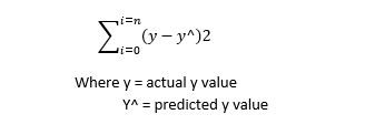
3. Measure the distance b/w all the points in the feature space and the line using the formula below

4. Now construct another line that should pass through Centroid but not the origin. Below diagram shows different lines that are possible.

5. Keep on repeating the process until you find the line with the minimum distance which will be your best fit line. Below fig. shows the best fit line.

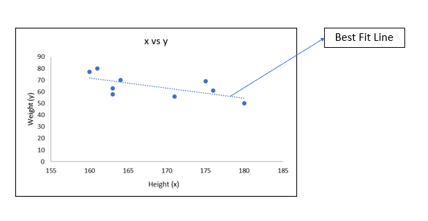
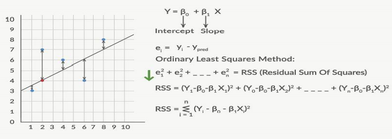
The best fit line will serve the purpose of being the predictor. It can be represented in the equation

Y^ =  mx  + c

where c (intercept) –  the point in the y-axis which the best fit line passes through
m – is the slope of the best fit line
x – is the input variable

For example, when a new person’s height(x) is inputted we will use this equation to find the prediction of weight(y)

Multiple linear regression follows the same process but instead of a line, it will be a plane. The process of finding the best-fit plane is the same as SLR but it will be in higher dimensions.

The equation for best fit plane will look like  Y^ =  c + m1*x1 + m2*x2 +…+ mn*xn

Assumptions

For linear regression to hold true and to use for business problems it should pass the four assumptions :

1. Linearity between x and y
2. Error terms are normally distributed
3. No multicollinearity
4. Equivalence of variance (Homoscedasticity)

Linearity between x and y

• This is the important assumption the dependent variable (x) should be linear related to the independent variable (y).
• Only then we will be able to perform linear regression on our data.
• Slopes should be linearly related to y and not x itself.

Error terms are normally distributed

• Once we fit the line and for our existing data, we will try to predict y.
• After that, we will find the difference between actual and predicted.
• Let’s if we have 100 samples. We will 100 predictions as well.
• We compute the difference between actual and predicted for these 100 samples and plot a histogram.
• If the distribution is normal then this assumption is cleared. Else linear regression cannot be used for interpretation.

No Multicollinearity

• This assumption comes into the picture only for multiple linear regression.
• This is assumption states that there should not be any high correlation between different independent variables.
• Correlation to some extent is tolerated. This can be verified using a technique called variance inflation factor (VIF).
• VIF is given by 1/(1-R2). We will see about VIF in detail in the next blog.
• Industry-standard VIF should be less than 5.

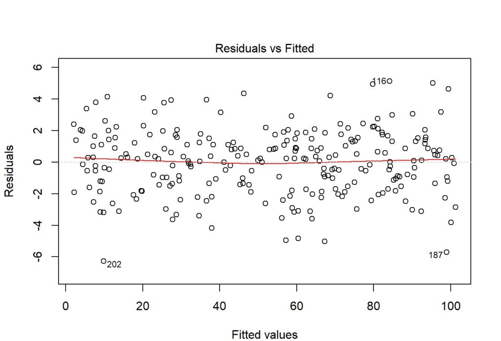
Equivalence of variance (Homoscedasticity)

• The scatter plot between error terms (residuals) and y actuals should be similar to what’s shown in the figure below.

Once all these assumptions are cleared. We will check the  significance of the dependent variables which should be done using a hypothesis test.

•     H₀: Variable is not significant
•     H_a: Variable is significant

If the p-value of a dependent variable is less than 0.05 it is significant else we should remove it from the model.
Industry-standard p-value should be less than 0.05 but depending on our application we can change increase or decrease this threshold.

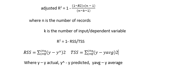
Checking Model Performance

Widely used metric to evaluate linear regression model is adjusted R-squared.

Summary

Linear Regression falls under Supervised Learning
It is broadly classified into Simple Linear Regression and Multiple Linear Regression.
Linear Regression has four assumptions and every assumptions need to pass for LR to hold good.
Popularly used metric to assess the model is adjusted R-square.

Watch out this space for step by step practical implementation of Linear Regression in Python.